¶ MODEL BUILDING
¶ 1. Linear regression
To build a linear regression, go to the column settings by clicking on the  icon. Then go to the “Models” tab (Fig. 1.1).
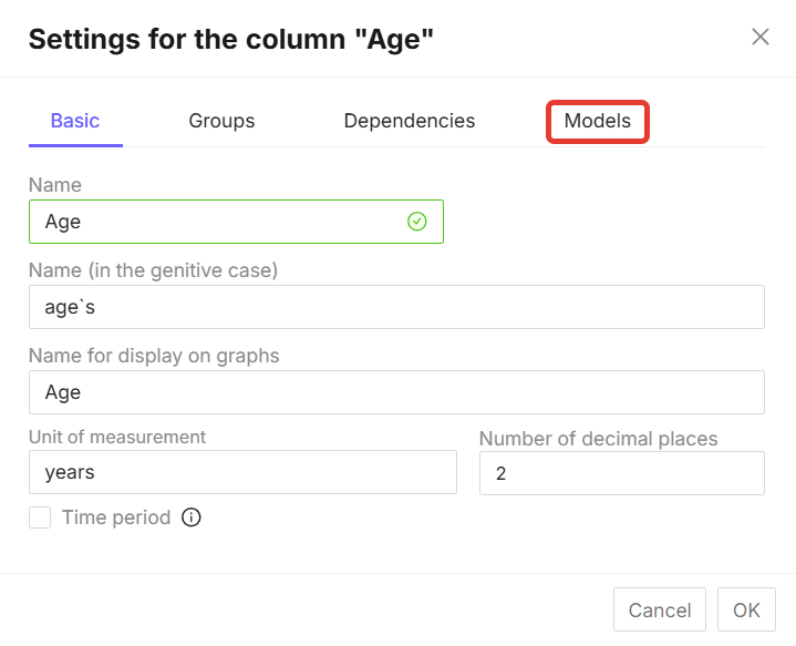
Figure 1.1 - “Models” tab in the column settings
This tab contains the model building functionality, which consists of “Predictor Selection” (Fig. 1.2) and “Independent Columns” selection (Fig. 1.3).
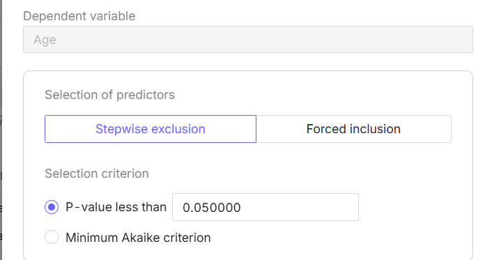
Figure 1.2 - “Predictor Selection” functionality
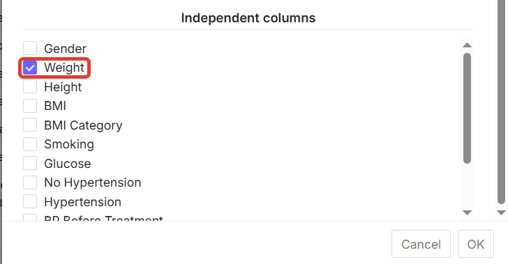
Figure 1.3 - Selecting independent columns for regression
When selecting predictors, you can use “Stepwise exclusion” to include only significant variables in the analysis. The selection criteria for “Stepwise exclusion” can be either “p-Value” or “Minimum Akaike criterion” (Fig. 1.4). And “Forced Inclusion” - all selected variables (columns) will be included in the analysis (Fig. 1.5).
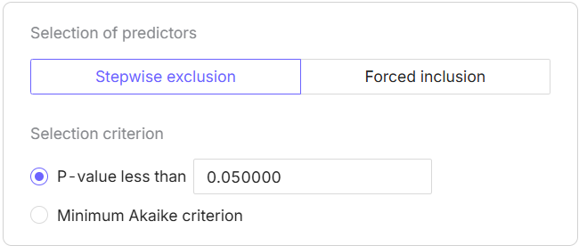
Figure 1.4 - “Selection criterion” in the “Models” tab

Figure 1.5 - “Forced inclusion” in the “Models” tab
To build a logistic regression, select the variable you want to analyze in the “Independent Columns” block on the “Models” tab. For example, let's build a predictive model that shows how blood pressure (BP) depends on a patient's age using linear regression.
To perform this analysis, select the “Age” indicator in the “Independent Columns” block in the “BP” column in the “Models” tab. Then click on the “OK” button (Fig. 1.6).
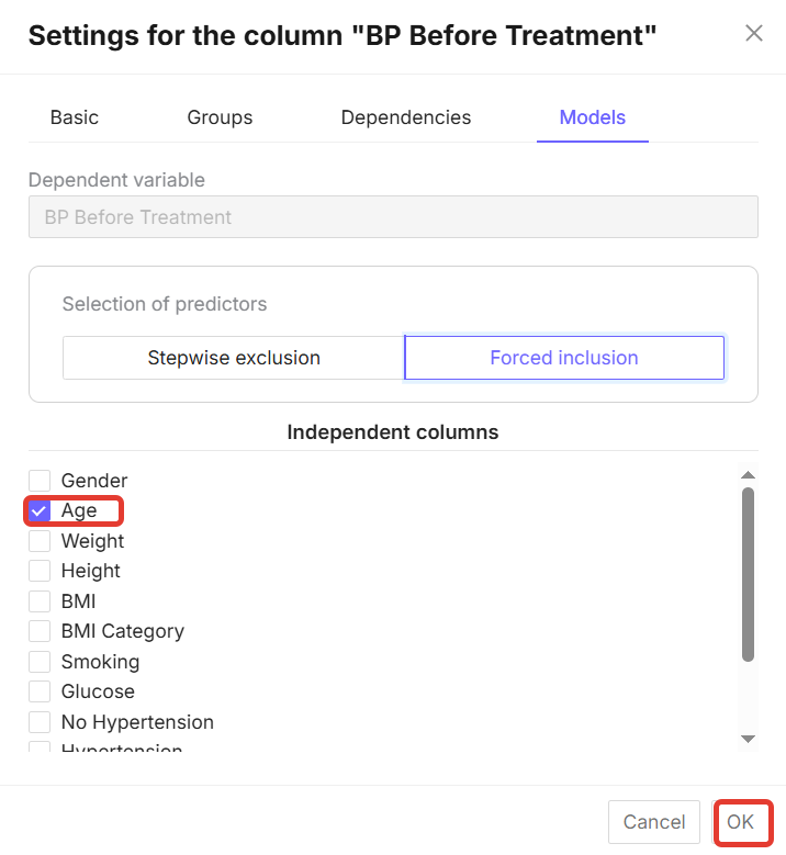
Figure 1.6 - Selecting an indicator in the “Models” tab
Next, click on the “Perform analysis” button in the upper right corner of the screen (Fig. 1.7).
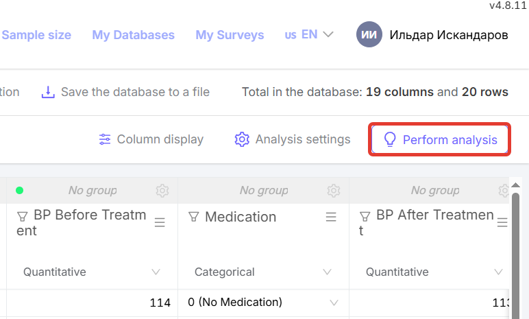
Figure 1.7 - “Perform analysis” button
The structure of the analysis will look as follows (Fig. 1.8).
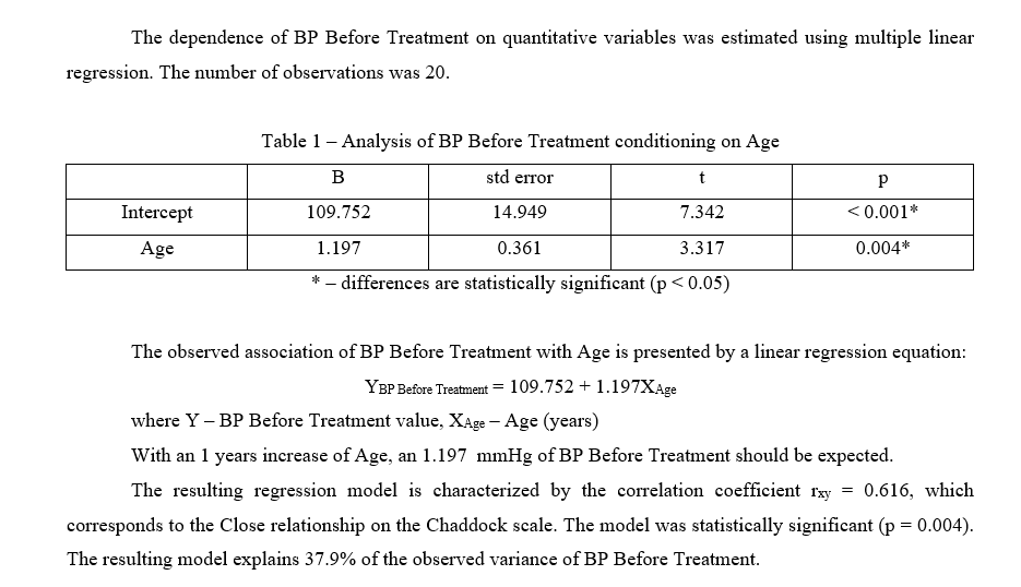
Figure 1.8 - Example of analysis output using the linear regression method.
This analysis can also be performed based on several factors. In this case, select several factors for analysis in the “Independent columns” section of the “Models” tab. (Fig. 1.9)
Figure 1.9 - Example of selecting several indicators for analysis
Next, click on the “Perform analysis” button (Fig. 1.7). The structure of the generated analysis looks as follows (Fig. 1.10).
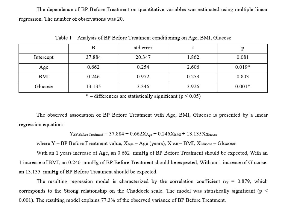
Figure 1.10 - Example of a generated multifactor analysis using the linear regression method
¶ 2. Logistic regression
To build a logistic regression, go to the column settings by clicking on the icon. Then go to the “Models” tab (Fig. 2.1).
This tab contains the model building functionality, which consists of “Predictor Selection” (Fig. 2.2) and “Independent Columns” selection (Fig. 2.3).
In predictor selection, you can use “Stepwise Elimination” to include only significant variables in the analysis. The selection criteria for “Stepwise exclusion” can be either “p-Value” or “Minimum Akaike criterion” (Fig. 2.4). And “Forced inclusion” - all selected variables (columns) will be included in the analysis (Fig. 2.5).
To build a logistic regression, select the necessary variable for analysis in the “Models” tab in the “Independent Columns” block. As an example, let's build a predictive model characterizing the dependence of blood pressure (BP) on patient age, smoking status, and body mass index (BMI) using the binary logistic regression method.
To perform this analysis, select the “Age,” “Smoking,” and “BMI” indicators in the “Independent Columns” block in the “Blood Pressure” column on the “Models” tab. Then click the “OK” button (Fig. 2.11).
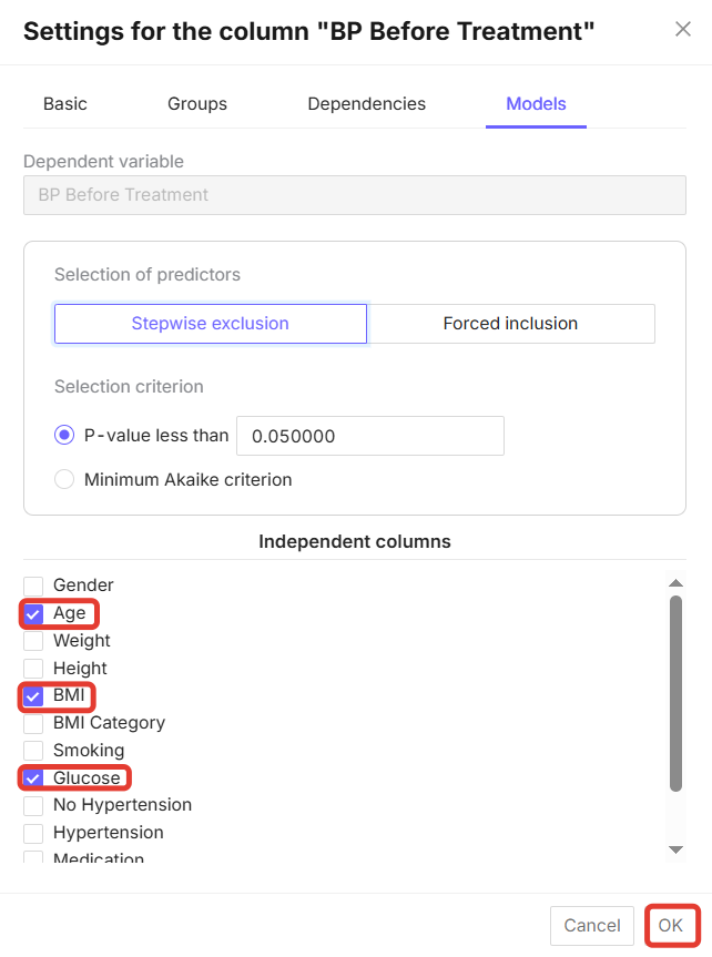
Figure 2.11 - Selecting variables in the “Models” tab
Next, click on the “Perform analysis” button in the upper right corner of the screen (Fig. 2.7).
The structure of the analysis will look as follows (Fig. 2.12 - Fig. 2.15).
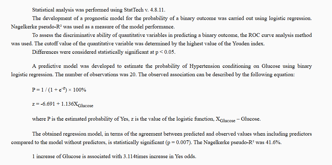
Figure 2.12 - Example of a developed predictive model and description of statistical analysis methods
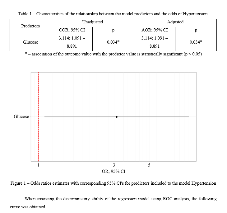
Figure 2.13 - Example of binary logistic regression output
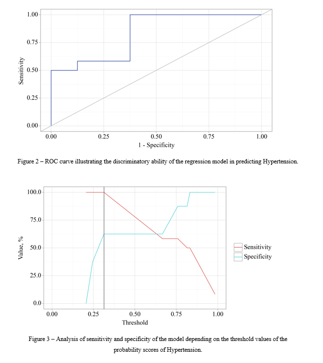
Figure 2.14 - Example of a ROC curve and analysis of the sensitivity and specificity of the constructed model
Figure 2.15 - Example of a table and output of threshold values of the logistic function
¶ 3. Survival analysis
To perform survival analysis, the database must contain an “Event” column. For example, a fatal outcome indicator. The column must have a binary distribution (0 - event occurred, 1 - event did not occur) (Fig. 3.1).
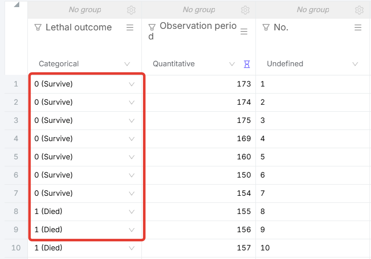
Figure 3.1 - Example of filling in the “Event” column - “Fatal outcome”
To perform survival analysis, you also need to create a column called “Observation period” - this is the period from the date to the “Event” or from the date to the last contact with the patient if the event did not occur. It is measured in weeks, months, years, or other time intervals (Fig. 3.2).
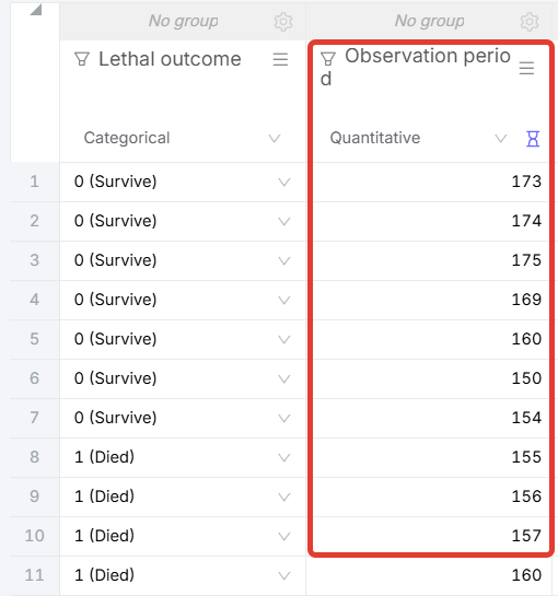
Figure 3.2 - Example of filling in the “Observation period” column
In order to analyze survival in the “Observation period” column, you need to check the box in the column settings for the “Time period” function. After activating the “Time period” function, a line with the “Survival type” selection will appear (Fig. 3.3).
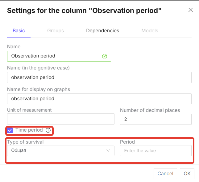
Figure 3.3 - “Time period” function in the column settings
Next, in the “Event” column, go to “Column Settings” - “Models” and select the necessary indicators for analysis in the “Independent Columns” block. “Observation Period” must always be specified. Then click the “OK” button (Fig. 3.4).
Figure 3.4 - Selecting indicators for “Events” analysis
Then click the “Perform analysis” button in the upper right corner of the page (Fig. 3.5).
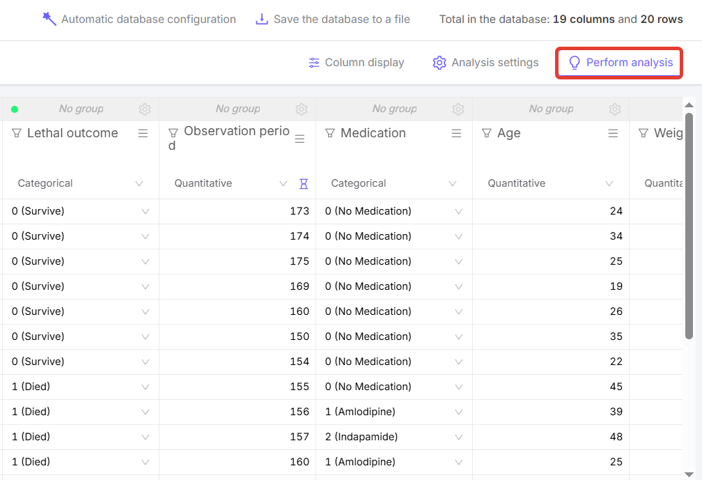
Figure 3.5 - “Perform analysis” button
Survival analysis can be single-factor, i.e., looking at the impact of only one factor on survival. One indicator is selected in the “Models” tab (Fig. 3.6). It can also be multi-factor, when several indicators are selected (Fig. 3.7).
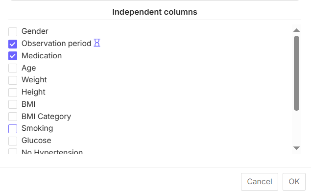
Figure 3.6 - Example of selecting one factor for analysis
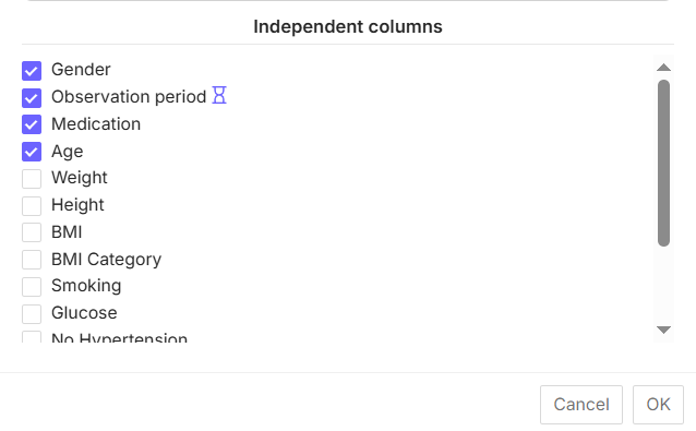
Figure 3.7 - Example of selecting several factors for analysis (multifactorial analysis)
The structure of survival analysis consists of:
- Description of statistical analysis methods (Fig. 3.8);
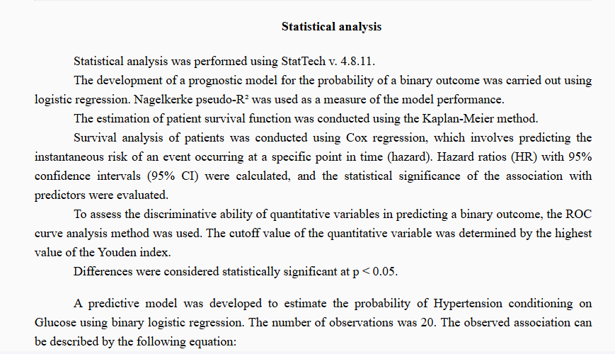
Figure 3.8 - Example of a description of statistical analysis methods
- Survival curve (Fig. 3.9). It is displayed only for categorical indicators;
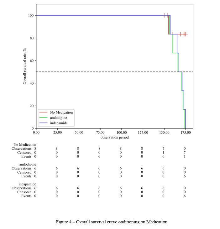
Figure 3.9 - Example of a survival curve
- Conclusion on the survival curve (Fig. 3.10);
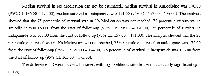
Figure 3.10 - Example of a conclusion on the survival curve
- Assessment of the relationship between survival and the factors under study using Cox regression (Fig. 3.11);
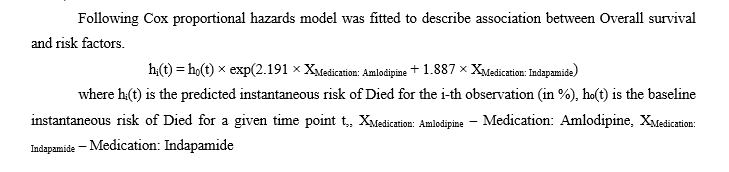
Figure 3.11 - Example of assessing the relationship between survival and the factors under study
- Table of baseline risk depending on time periods (Fig. 3.12);
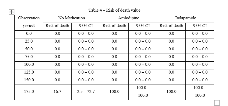
Figure 3.12 - Example of a basic risk table
- Table of risk changes depending on the factors under study (Fig. 3.13);
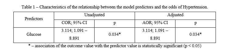
Figure 3.13 - Example of a risk table depending on the influence of factors
- Graph of risk ratio assessment with 95% CI for the factors under study (Fig. 3.14);
Figure 3.14 - Example of a risk ratio assessment graph
- Tables of recurrence-free survival values (Fig. 3.15).
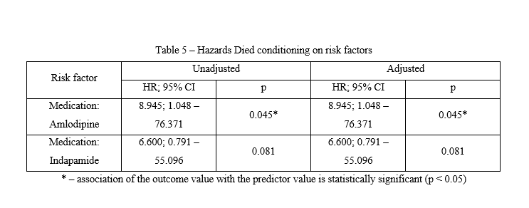
Figure 3.15 - Table of recurrence-free survival values
¶ 4. Time series
To analyze and construct time series, the database must contain a column with the phenomenon (e.g., number of deaths) and a column with the time period (e.g., years).
In the “Years” column, go to the column settings and set the time period attribute (Fig. 4.1).
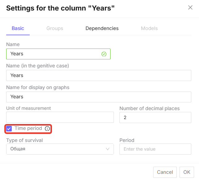
Figure 4.1 - “Time period” function
Then go to the “Dependencies” tab and check the box next to the event column, in this case, “Number of deaths,” and click the “OK” button (Fig. 4.2).
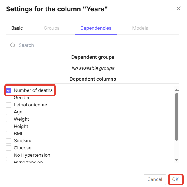
Figure 4.2 - Selecting a dependent column for building dynamic series
Next, click the “Perform analysis” button in the upper right corner of the page (Fig. 4.3).
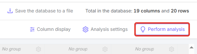
Figure 4.3 - “Perform analysis” button
The completed analysis will consist of a table analyzing the dynamics of the indicator with the event (Fig. 4.4), a text output (Fig. 4.5), and a diagram (Fig. 4.6).
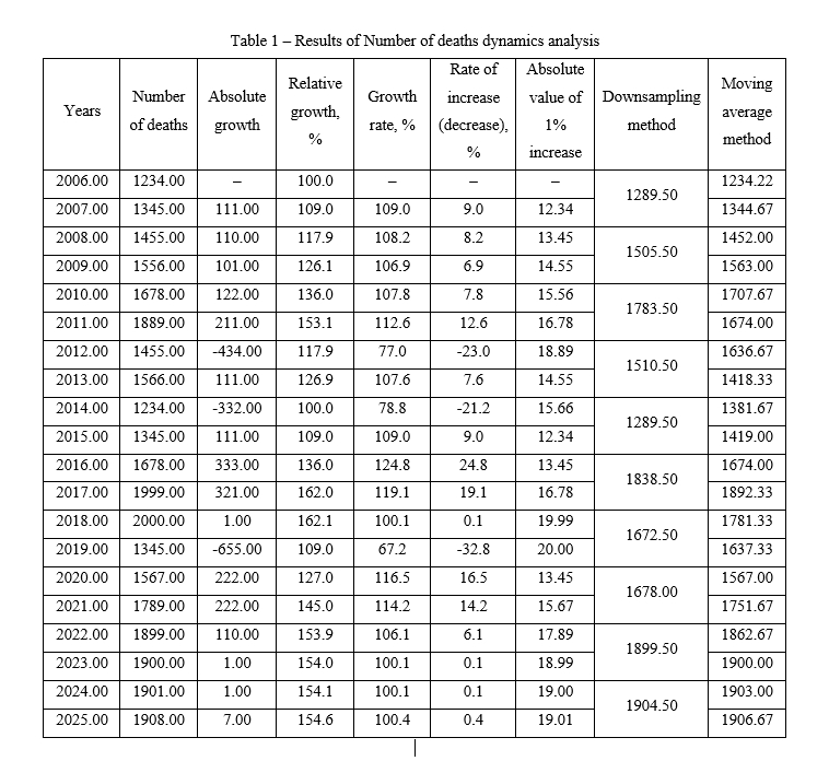
Figure 4.4 - Tabular form of data analysis
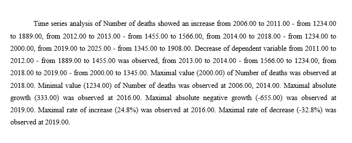
Figure 4.5 - Text output for data analysis
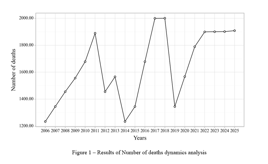
Figure 4.6 - Data analysis diagram
¶ 5. Calculating variables
To calculate variables, click the button in the top row of the database window (Fig. 5.7).
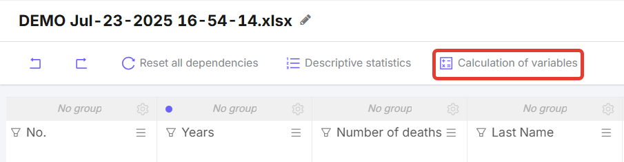
Figure 5.7 - “Calculate variables” button
After clicking, a window resembling a calculator opens, with “Variables” (columns from the database) on the left and calculation functions on the right (Fig. 5.8).
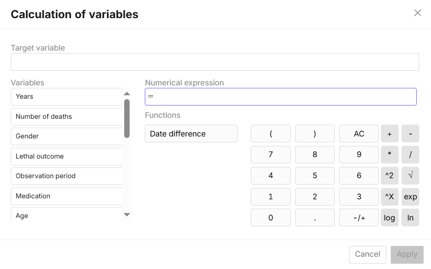
Figure 5.8 - “Calculate variables” window
Table of keys for calculating variables
 |
Button to clear the line "Numeric expression" |
 |
Addition of variables (numbers) |
 |
Subtraction of variables (numbers) |
 |
Multiplication of variables (numbers) |
 |
Division of variables (numbers) |
 |
Square of a variable (number) |
 |
Square root of a variable (number) |
 |
Raising to a certain power |
 |
Calculating the exponent |
 |
Common logarithm function |
 |
Natural logarithm function |
 |
Allows you to change the current positive number to negative, and vice versa |
 |
Date difference function
|
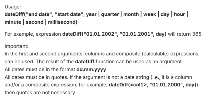
Figure 5.9 - Rules for using the “Date difference” function
In the “Target variable” line, enter the name of the column in which the new variable will be calculated. In the “Numerical expression” line, enter the formula for the calculation. For example, to calculate height in meters, take the “Height” column already in the database and divide it by 100. To complete the calculation, click the “Apply” button (Fig. 5.10.
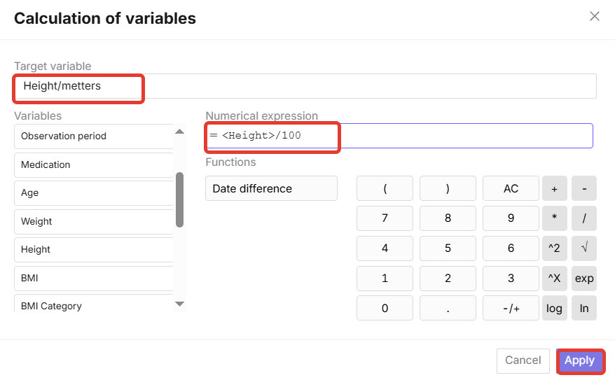
Figure 5.10 - Example of calculating a new variable
The new column is added to the end of the database (Fig. 5.11). These columns will always have a quantitative variable type.
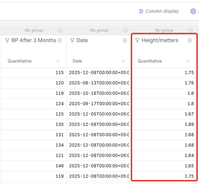
Figure 5.11 - Example of a calculated column created in the database